Compositional Multilevel Substitution Models • multilevelcoda

Intro

We often are interested in how an outcome changes when a fixed unit of the predictor (e.g., minutes of behaviours during a day) is reallocated from one compositional component to another. The Compositional Isotemporal Substitution Model can be used to estimate this change. The multilevelcoda package implements this method in a multilevel framework and offers functions for both between- and within-person levels of variability. We discuss 4 different substitution models in this vignette.

We will begin by loading necessary packages, multilevelcoda, brms (for models fitting), doFuture (for parallelisation), and data sets mcompd (simulated compositional sleep and wake variables), sbp (sequential binary partition), and psub (base possible substitution).

library(multilevelcoda)
library(brms)
library(doFuture)

data("mcompd") 
data("sbp")
data("psub")

options(digits = 3) # reduce number of digits shown

Fitting main model

Let’s fit our main brms model predicting STRESS from both between and within-person sleep-wake behaviours (represented by isometric log ratio coordinates), with sex as a covariate, using the brmcoda() function. We can compute ILR coordinate predictors using compilr() function.

cilr <- compilr(data = mcompd, sbp = sbp,
                parts = c("TST", "WAKE", "MVPA", "LPA", "SB"), idvar = "ID")

m <- brmcoda(compilr = cilr,
             formula = STRESS ~ bilr1 + bilr2 + bilr3 + bilr4 +
                                wilr1 + wilr2 + wilr3 + wilr4 + Female + (1 | ID),
             cores = 8, seed = 123, backend = "cmdstanr")

A summary() of the model results.

summary(m$Model)
#>  Family: gaussian 
#>   Links: mu = identity; sigma = identity 
#> Formula: STRESS ~ bilr1 + bilr2 + bilr3 + bilr4 + wilr1 + wilr2 + wilr3 + wilr4 + Female + (1 | ID) 
#>    Data: tmp (Number of observations: 3540) 
#>   Draws: 4 chains, each with iter = 2000; warmup = 1000; thin = 1;
#>          total post-warmup draws = 4000
#> 
#> Group-Level Effects: 
#> ~ID (Number of levels: 266) 
#>               Estimate Est.Error l-95% CI u-95% CI Rhat Bulk_ESS
#> sd(Intercept)     0.99      0.06     0.87     1.11 1.00     1179
#>               Tail_ESS
#> sd(Intercept)     2176
#> 
#> Population-Level Effects: 
#>           Estimate Est.Error l-95% CI u-95% CI Rhat Bulk_ESS
#> Intercept     2.64      0.47     1.68     3.57 1.00     1429
#> bilr1         0.12      0.33    -0.54     0.77 1.00      971
#> bilr2         0.53      0.35    -0.16     1.21 1.00     1124
#> bilr3         0.13      0.21    -0.29     0.55 1.00     1052
#> bilr4        -0.01      0.29    -0.57     0.55 1.00     1021
#> wilr1        -0.34      0.12    -0.58    -0.10 1.00     2990
#> wilr2         0.05      0.13    -0.21     0.31 1.00     3396
#> wilr3        -0.10      0.08    -0.25     0.04 1.00     2900
#> wilr4         0.23      0.10     0.04     0.43 1.00     2894
#> Female       -0.39      0.17    -0.74    -0.08 1.00     1405
#>           Tail_ESS
#> Intercept     2263
#> bilr1         1409
#> bilr2         1679
#> bilr3         1809
#> bilr4         1941
#> wilr1         3206
#> wilr2         3077
#> wilr3         3218
#> wilr4         3220
#> Female        1697
#> 
#> Family Specific Parameters: 
#>       Estimate Est.Error l-95% CI u-95% CI Rhat Bulk_ESS Tail_ESS
#> sigma     2.37      0.03     2.31     2.43 1.00     4462     2814
#> 
#> Draws were sampled using sample(hmc). For each parameter, Bulk_ESS
#> and Tail_ESS are effective sample size measures, and Rhat is the potential
#> scale reduction factor on split chains (at convergence, Rhat = 1).

We can see that the first and forth within-person ILR coordinates were both associated with stress. Interpretation for multilevel ILR coordinates can often be less intuitive. For example, the significant coefficient for wilr1 shows that the within-person change in sleep behaviours (sleep duration and time awake in bed combined), relative to wake behaviours (moderate to vigorous physical activity, light physical activity, and sedentary behaviour) on a given day, is associated with stress. However, as there are several behaviours involved in this coordinate, we don’t know the within-person change in which of them drives the association. It could be the change in sleep, such that people sleep more than their own average on a given day, but it could also be the change in time awake. Further, we don’t know about the specific changes in time spent across behaviours. That is, if people sleep more, what behaviour do they spend less time in?

This is common issue when working with multilevel compositional data as ILR coordinates often contains information about multiple compositional components. To gain further insights into these associations and help with interpretation, we can conduct post-hoc analyses using the substitution models from our multilevel package.

Substitution models

multilevelcoda package provides 2 different methods to compute substitution models, via the substitution() function.

Basic substitution models:

Between-person substitution
Within-person substitution

Average marginal substitution models:

Average marginal between-person substitution
Average marginal within-person substitution

Tips: Substitution models are often computationally demanding tasks. You can speed up the models using parallel execution, for example, using doFuture package.

Basic Substitution model

The below example examines the changes in stress for different pairwise substitution of sleep-wake behaviours for a period of 1 to 5 minutes, at between-person level. We specify level = between to indicate substitutional change would be at the between-person level, and ref = "grandmean" to indicate substitution model using the grand compositional mean as reference composition. If your model contains covariates, substitution() will average predictions across levels of covariates as the default.

subm1 <- substitution(object = m, delta = 1:10,
                      ref = "grandmean", level = c("between", "within"))

Output from substitution() contains multiple data set of results for all available compositional component. Here are the results for changes in stress when sleep (TST) is substituted for 10 minutes.

knitr::kable(summary(subm1, delta = 10, level = "between", to = "TST"))

Mean	CI_low	CI_high	Delta	From	To	Level	Reference
0.06	0.00	0.13	10	WAKE	TST	between	grandmean
0.00	-0.03	0.04	10	MVPA	TST	between	grandmean
0.01	-0.01	0.04	10	LPA	TST	between	grandmean
0.01	-0.02	0.04	10	SB	TST	between	grandmean

None of them are significant, given that the credible intervals did not cross 0, showing that increasing sleep (TST) at the expense of any other behaviours was not associated in changes in stress at between-person level. These results can be plotted to see the patterns more easily using the plotsub() function.

plotsub(data = subm1$BetweenSub$TST, 
        x = "sleep", y = "stress")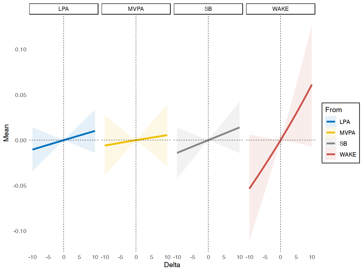

Example of Between-person Substitution Model

Here are the results for within-person level.

knitr::kable(summary(subm1, delta = 10, level = "within", to = "TST"))

Mean	CI_low	CI_high	Delta	From	To	Level	Reference
0.04	0.00	0.07	10	WAKE	TST	within	grandmean
-0.01	-0.02	0.01	10	MVPA	TST	within	grandmean
-0.01	-0.02	0.00	10	LPA	TST	within	grandmean
0.00	-0.01	0.01	10	SB	TST	within	grandmean

At within-person level, we got some significant results for substitution of sleep (TST) and time awake in bed (WAKE) for 5 minutes, but not other behaviours. Increasing 5 minutes in sleep at the expense of time spent awake in bed predicted 0.04 higher stress [95% CI 0.01, 0.7], on a given day. Conversely, less sleep and more time awake in bed predicted less stress (b = -0.03 [95% CI -0.06, -0.01]). Let’s also plot theses results.

plotsub(data = subm1$WithinSub$TST, x = "sleep", y = "stress")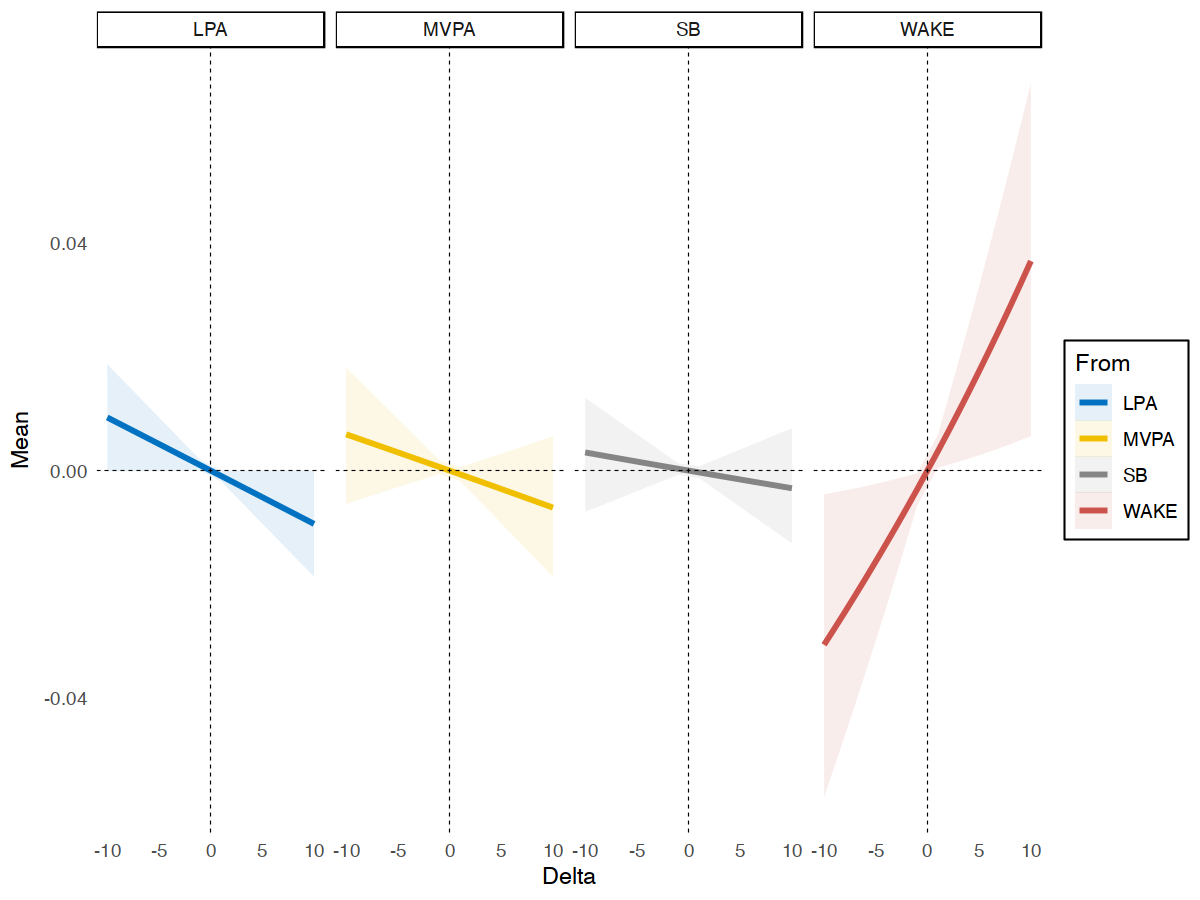

Example of Within-person Substitution Model

Average Marginal Substitution Effects

The average marginal models use the unit compositional mean as the reference composition to obtain the average of the predicted group-level changes in the outcome when every unit (e.g., individual) in the sample reallocates a specific unit from one compositional part to another. This is difference from the basic substitution model which yields prediction conditioned on an “average” person in the data set (e.g., by using the grand compositional mean as the reference composition). Average substitution models models are generally more computationally expensive than basic subsitution models. All models can be run faster in shorter walltime using parallel execution. In this example, we use package doFuture to parallel our models. substitution() will run 5 substitution models for 5 sleep-wake behaviours, so we will parallel them across 5 workers.

registerDoFuture()
plan(multisession, workers = 5)

subm2 <- substitution(object = m, delta = 1:10,
                      ref = "clustermean", level = c("between", "within"))
registerDoSEQ()

Below are the results.

knitr::kable(summary(subm2, delta = 10, to = "TST"))

Mean	CI_low	CI_high	Delta	To	From	Level	Reference
0.09	-0.05	0.24	10	TST	WAKE	between	clustermean
0.02	-0.10	0.15	10	TST	MVPA	between	clustermean
0.03	-0.09	0.15	10	TST	LPA	between	clustermean
0.03	-0.09	0.15	10	TST	SB	between	clustermean
0.05	0.01	0.08	10	TST	WAKE	within	clustermean
-0.01	-0.02	0.01	10	TST	MVPA	within	clustermean
-0.01	-0.02	0.00	10	TST	LPA	within	clustermean
0.00	-0.01	0.01	10	TST	SB	within	clustermean

A comparison between between- and within-person substitution model of sleep on stress, plot using plotsub() and ggpubr::ggarrange() functions.

library(ggpubr)
p1 <- plotsub(data = subm2$BetweenSubMargins$TST, x = "between-person sleep", y = "stress")
p2 <- plotsub(data = subm2$WithinSubMargins$TST, x = "within-person sleep", y = "stress")

ggarrange(p1, p2, 
          ncol = 1, nrow = 2)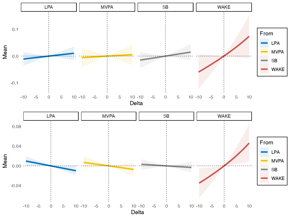

Example of Average Marginal Substitution Model